The purpose of the physical fates submodel is to estimate the distribution in three physical dimensions plus time of a contaminant on the water surface, along shorelines, in the water column, and in the sediments. The logical structure of this submodel, and its relationship to the geographical information system (GIS), chemical database, and the biological effects submodel are shown in Figure 1.2. The user supplies a spill location for a specific application of the NRDAM/CME. The GIS then supplies fixed grids necessary for the simulation. The chemical database supplies chemical parameters required by the submodel. The user is required to supply a wind time series specific to the time and location of the spill.

 If the specific gravity of a spilled substance is less than or equal to that of water, the model employs surface spreading, advection, entrainment, and volatilization algorithms to determine transport and fate at the surface. A contaminant with specific gravity greater than water is modeled by a convective jet algorithm which allows the contaminant plume to reach an equilibrium position in a stratified water column, or to sink to the bottom. In general, some fraction of any contaminant spilled will exist in both the water column and the sediments. In the water column, horizontal and vertical advection and dispersion are simulated by random walk procedures. Partitioning between particulate-adsorbed and dissolved states is calculated based on linear equilibrium theory. The contaminant fraction that is adsorbed to suspended particulate matter is assumed to settle at a rate typical for the environment. Contaminants at the bottom are mixed into the underlying sediments according to a simple bioturbation equation. Degradation in water and sediments is requested as a first order decay process.

 The model is designed to simulate fates of pure hazardous substances, crude oils, and petroleum products. These latter are actually complex mixtures of hydrocarbons. For modeling purposes, crude oils and petroleum products are represented by four components:

　

 Toxicity in the water column is associated only with the aromatic fractions, consistent with the derivation of effects levels for petroleum substances, as discussed in Section 4.

 The physical environment is divided into six general compartments: the atmosphere, the water surface, the upper and lower water columns (as defined by the presence or absence of a pycnocline at the base of a surface mixed layer), the bottom, and the shoreline. The submodel distributes a contaminant dynamically in three physical dimensions among these compartments. Only the atmospheric compartment has no physical representation and no linkage to the biological effects submodel.

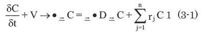
 The model solves the generalized transport equation:

　

　

 On the water surface and the shoreline, "concentration" C has units of mass per unit area, whereas in the water column and sediments the units are mass per unit volume, and

　

　

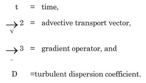
 The objective in solving Equation 3-1 is to produce for the biological effects submodel a spatial time-history of the distribution of a contaminant in the environment. The first term on the left hand side is the temporal rate of change of the concentration at a particular location in space. This rate of change is computed in the submodel by solving the other terms in Equation 3-1: the second term on the left (the advective transport term); the first term on the right (the diffusive transport term); the series of process-specific terms at the end of the equation.

　

 Equation 3-1 is central to the physical fates submodel in that it summarizes all the processes simulated therein. The algorithms used to simulate these processes controlling physical fates of substances are described in detail below. In general, equations are given as in the original references, and units are converted within the model code itself.

　

 The major assumptions in the physical fates submodel are discussed below.

　

 The model accepts as input a single time series, with no allowance for spatial variability. For spills which cover large areas, traverse great distances, or occur in very mountainous areas where orographic effects are important, results may diverge from reality. (This effect can be ameliorated by concatenating wind time series corresponding to the geographic area in which the major portion of a spill is found at subsequent times during an event.)

　

 The currents in the model are two dimensional, vertically averaged values. In reality, wind stress at the water surface propagates downward by turbulence, producing in general a velocity shear near the surface. Three-dimensional complexities such as reverse flows at depth, vertical shear profiles, upwelling and downwelling are inherently neglected in the present version of the NRDAM/CME. This means that both the magnitude and direction of transport vectors in the water column may be in error. The ultimate effect of errors in transport velocities on the reliability of the damage figure, however, is probably least in offshore areas, since the biological habitats tend to be homogeneous offshore.

　

 The physical fates submodel resolves the physical domain into discrete rectangular grid cells, with attributes being uniform within a cell. Increasing the resolution, by using more, smaller cells, provides a better representation of the real world as long as reliable data at the finer resolution is available. The NRDAM/CME has a resolution of 1 to 10 km, commensurate with available data for bathymetry, shoreline type, and currents. Higher resolution is used in nearshore areas, with broader scales offshore.

　

 The model represents contaminant distributions on the water surface and in the water column by distributions of discrete slicks or particles. The maximum number of slicks and particles allowed by the computational software/hardware affects the ability of the model to resolve these spatial distributions. For longer or more chronic spills, the limited number of available slicks and particles results in less precise resolution. The model is designed to adequately resolve contaminant releases of up to a few days in duration.

　

 The fates submodel uses individual particles to simulate the transport of contaminants in the water column. A fraction of the contaminant mass is associated with each particle. These particles are Lagrangian in the sense that they move with the surrounding water. The use of Lagrangian particles in the contaminant transport calculations effectively eliminates numerical diffusion problems associated with finite difference calculations in the presence of steep gradients (e.g. at the edge of contaminant plumes), and also provides a more versatile modeling framework.

 An expanding, translating 3-dimensional grid system is used to resolve concentration levels in the water column. At each timestep for which water column concentrations are to be output to the biological submodel, the Lagrangian grid is "stretched" in the vertical and horizontal dimensions until all contaminant particles are within the grid boundaries, at which time concentrations are computed within each three dimensional grid cell. This expanding grid allows the model to resolve a wide range of spill sizes, and eliminates the interdependence between the dimensions of the Eulerian (fixed) transport grid and the magnitude of the spill.

　

 The spreading of pollutant spills on the water surface occurs due to current shears in both the horizontal and vertical dimensions. In addition, local spreading is computed based on the gravity - viscous formulation of Fay (1971) and Hoult (1972) as modified empirically by Mackay et al., (1980). The rate of change of surface area with time is

dA/dt = K1A^1/3(Vm/A)^3/44　(3-2)

in which

　

 The first (gravity - inertial) phase in the Fay - Hoult spreading theory is of short duration, and is not accounted for in Equation (3-2). The radial spreading rate is therefore limited here to a maximum of 0.1 m/sec, a mean value for the duration of the first regime for a 100 m³ oil spill (Dippner, 1983). The spreading process ceases at a specified terminal thickness. The spreading rate constant K1 is set to 5.0 x 10⁸ per day, based on observations by Audunson et al. (1984), Sørstrøm and Johansen (1985), JBF (1976), Sørstrøm (1989), and Reed et al (1990, 1992).

　

 For surface volatilization, the methodology of Mackay and Matsugu (1973) is adopted, in which the mass transfer coefficient, K1 (m/hr), is computed as

　

　

where

　

 Following Mackay et al., (1980), we use the Schmidt number, Sc, for cumene, 2.7. The molecular weight term in (3-3) is a diffusivity correction in air from Payne et al., (1984). The mass transfer rate (gm/hr) from the surface slick is then

dm/dt = (K2PvpA/RT) FMW6　(3-4)

where

　

 As discussed earlier, the volatile fraction of mixtures such as crude oil and petroleum products is defined here as the sum of three fractions:

　

 For compounds, the mass-weighted mean molecular weight of the substance is used in Equations 3-3 and 3-4.