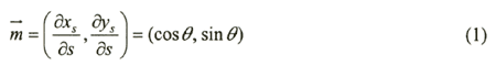
We used the shoreline evolution model using the curvilinear coordinate system of Suh and Hardaway (1994). The curvilinear coordinate system of the model is shown in Figure 6 along with some other notations. The symbol s denotes the coordinate following the shoreline. The coordinate pair (x_s, y_s ) gives the location of an arbitrary point on the curved shoreline in terms of a Cartesian coordinate system.

　

　

is the unit tangential vector to the shoreline in the direction of increasing s,

　

　

is the seaward unit normal vector to the shoreline, and θ is the angle between and the x - axis which is measured counterclockwise from the positive x -direction. In the figure, Q is the volumetric sediment transport rate, and α_b is the breaking wave angle between the wave crest and the x -axis, which is measured counterclockwise from the positive x -direction. Assuming that the point, (x_s, y_s), moves perpendicular to the shoreline, so that

　

　

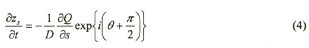
in which e = -(1/D )∂Q / ∂s (D = depth of profile closure) is the rate of shore-normal movement of shoreline, and introducing z_s = x_s + iy_s, in which , the preceding equation can be written as

　

　

　

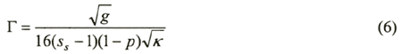
The longshore sediment transport rate formula proposed by Ozasa and Brampton (1980) is used, which includes the effect of wave diffraction on longshore sediment transport:

　

　

in which

　

　

and

　

　

is the breaking wave angle relative to the shoreline under the assumption that the breaker line and the shoreline are locally parallel, and g = gravitational acceleration; s_s = specific gravity of sediment relative to fluid; p = porosity of sediment; κ = ratio of wave height to water depth at breaking; H_b = breaking wave height; tan β= beach slope; and K₁ , K₂ = empirical longshore sediment transport coefficients. An explicit finite-difference method is used to solve Equations (4), (5) and (7) numerically for the wave condition computed along the shoreline. See Suh and Hardaway (1994) for the finite-difference equations.

　

　

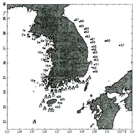
The sediment continuity equation (4), can be solved for the shoreline position, z_s, if the wave heights and angles along the breaker line are given. To calculate these, the RCPWAVE model developed by Ebersole et al. (1986) was used, which computes the wave transformation due to shoaling, refraction, and diffraction over an arbitrary bathymetry. For the offshore boundary condition of the wave model, we used the wave hindcasting data provided on the homepage of the Korea Ocean Research and Development Institute (http://www.kordi.re.kr). The deepwater wave hindcasting was made every three hours for 20 years (from 1979 till 1998) using the HYPA (Hybrid Parametric) model and the ECMWF (European Center for Medium-range Weather Forecasts) wind data. The site provides statistical data including significant wave height and period, principal wave direction, and directional wave spectrum at 67 locations around South Korea as shown in Figure 7. We used the data at Location 50 for three years from September 1979 to October 1982.

　

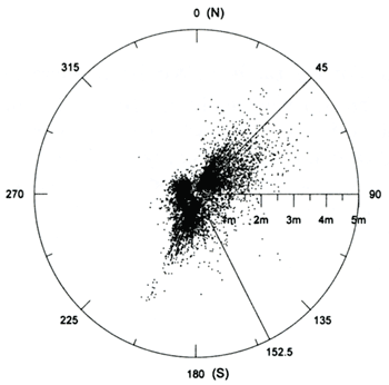
Figure 8 shows the distribution of heights and directions of the waves at Location 50. In the simulation, we used wave data in the sector between 45°and 152.5°clockwise from the north. Also we used only the waves of significant period greater than 4.0 s. The largest significant wave height is almost 5 m. The waves in the sector between NE and ENE are dominant.

　

　

　

The wave model uses Cartesian coordinate system with fixed grid spacing in both x and y directions. But the shoreline evolution model uses a curvilinear coordinate system in which the shoreline points move in both x and y directions, so that the spacing between shoreline points in x -direction is not constant even though we have a constant spacing at the beginning of the simulation. In order to calculate the breaking wave height and angle of a shoreline point, we took the weighting average of the values calculated at the neighboring points of the wave model. The detailed procedure can be found in Oh (2002).