The initial conditions for displacement and velocity are both assumed zero, i,e. xi(0)=0 and yi(0) = 0, Time interval is chosen as 120 and a time step 儮t = 1 is used, i.e. N = 120. Therefore a total of 240 unknown discretized external forces are to be determined in the present study. The number of measured displacements for system 1 and 2 are both 120.
(A) Numerical test case 1
The parameters that used in the test case 1 are taken as:
M1 = 1.0, M2 = 3.0, K1(t) = 4.0 + 0.01*t, K2(t) = 6.0 - 0.01*t,
C1(t) = 3.0+0.01*t and C2(t) = 5.0-0.01*t

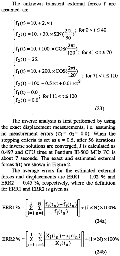
From those figures we concluded that the present algorithm has been applied successfully in the inverse vibration problem in estimating external forces since the estimated results are very accurate.
Next, let us discuss the influence of the measurement errors on the inverse solutions. When the measurement error for the displacements measured by sensors for subsystem 1 and 2 are taken as 冃1 = 0.07 (about 1 % of the average measured displacement for subsystem 1) and 02 = 0.13 (about 1 % of the average measured displacement for subsystem 2 ), then the stopping criteria 兠 can be calculated from equation (21). After 39 iterations (CPU time is about 5 seconds), the inverse solutions can be obtained and plotted in Figure 3 for the exact and estimated external forces. The average errors for the estimated external forces and displacements are ERR1 = 2.63 % and ERR2 = 1.35 %, respectively.
Then, the measurement error is increased to 冃1 = 0.35 (about 5 % of the average measured displacement for subsystem 1) and 02 = 0.65 (about 5 % of the average measured displacement for subsystem 2). After 14 iterations (CPU time is about 2 seconds), the inverse solutions can be obtained. In Figure 4 the exact and estimated external forces are shown. The average errors for the estimated extemal forces and displacements are ERR1 = 7,04 % and ERR2 = 8.76 %, respectively.
From the above Figures and data we learned that reliable inverse solutions can still be obtained when the large measurement errors are considered
丂
(B) Numerical test case 2
The parameters that used in the test case I are taken as:
M1 = 1.0, M2 = 2.0, K1(t) = 2.0 + 0.01* t, K2(t) = 3.0 - 0.01*t,
C1(t) = 1.0+0.01*t and C2(t) = 2.0-0.01*t
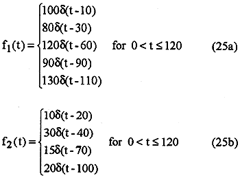
The unknown transient external forces fi(t) and f2(t) are assumed as the impulse function, which means large external forces will be applied to the system for only certain short time and forces remain zero for the rest of time. The impulse function can be expressed as:

Where 兟(丒) is the Dirac-deltafunction. The inverse analysis is first performed by using exact displacement measurements, i.e. assuming no measurement errors (冃i= 冃2= 0.0). When the stopping criteria is set as 8 = 1.2, after 87 iterations the inverse solutions are converged, J is calculated as 1.19 and CPU time is about 10 seconds. The exact and estimated external forces are shown in Figure 5 . From that Figure we know that for this strict test the estimated external forces are still very accurate.
Next, when the measurement error for the displacements measured by sensors for subsystem 1 and 2 are taken as 冃i = 0.09 (about 5 % of the average measured displacement for subsystem 1 ) and 冃2 = 0.1 (about 5 % of the average measured displacement for subsystem 2).