To apply our model we need to choose the observational values of only three parameters; we shall use Δρ₁, H₁ and H₂ because these are the three parameters that appear explicitly in our migration formula (7). Note that the numerical choices for these variables need to be made with care in the sense that, for consistency, we can only choose those values that lie within the validity regime of our model. Our choices [based on the observed maximum density gradient for the lower interface and a fairly arbitrary choice for the upper interface (see shaded and hatched regions in Fig. 2)] are,

　

(b)　The computed values

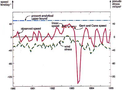
With our solution (6), (4), (1) and (7), the chosen numerical values give a pool thickness H of about 55m, a density difference Δρ₂ of 0.0026 gr/cm³, a speed under pool U² of -1.05ms^-1, and a migration rate C of 0.55ms^-1 (or 48km day^-1). (Recall that all of the results previously described for a cold pool on the bottom are equally applicable to a warm pool on top.) All of these values are very reasonable. For clarity, we show in Fig. 4 the predicted maximum migration speed C, the observed speed, as well as the speed predicted by hypothetical drifters released in the numerical model of Gent and Cane (see e.g., Murtugudde et al. 1996; Picaut et al. 1996) and in the earlier linear model (Cane and Patton 1984). The migration speed of the pool in the Gent and Cane model is very close to that of the linear model; both are about 40% lower than our analytically predicted upper bound and 15% or so lower than the observed speed.

Fig. 4.　A comparison of the observed pool's drift (solid line) to the theoretically predicted speed (dashed dotted line) and earlier predictions by the Gent and Cane model (long broken line) and the linear equatorial models (dashed double-dotted line). All are given in km/day. The pseudo stress (in m²s^-2) [which was averaged from COADS over a rectangular extending from 170°E to 160°W (15 degrees east and west of the pool's head mean position) and 4°S to 4°N] is also shown (short broken line). Note that the wind diminished completely during the 1982 El Nino, and that, during this year, the observed speed was about 25% lower than the new thoretical prediction and 10% higher than the values given by both Gent and Cane's model and the linear models. The observed position was averaged from 4°N to 4°S. (Aside from our newly computed upper bound, all values are reproduced from the unfiltered data of Picaut and Delcroix 1995 and Picaut et al. 1996).

BACK　　　CONTENTS　　　NEXT