|
NEURAL NETWORK APPROACH
The neural network approach, which has been developed in recently, is based on the concept of learning activities, such that, the procedure itself evolves an optimal model relating key variables.
| (Enlarge: 17KB) |
 |
| (Enlarge: 31KB) |
 |
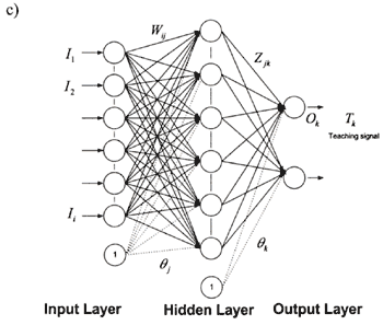
Figure 5. The architecture of a typical back-propagation neural network:
The output cell of perception (a), sigmoid function (b), and simple 3-layer neural network (c).
Neural network computing differs from artificial intelligence and traditional
computing in several important ways. Unlike traditional expert systems where the knowledge is made explicit
in the form of rules, neural networks generate their own rules by learning from the examples shown to
them. Learning is activated through a learning rule, which adapts or changes the connection weights of
the network in response to the example inputs and the desired outputs to those inputs. Learning in neural
networks refers to the processes of acquiring a desired behavior by changing the connection weights. Therefore,
the advantage of neural networks is that no subjective information is required to determine the model
structure or estimate parameters. Thus in analyzing large data sets with no a priori knowledge of processes
or causality the neural network is more a pragmatic approach. However, in terms of representing processes
neural networks will be severely limited. Only generalized process statements could be made from the neural
network models and for a process interpretation of algal growth behavior the dynamic mass balance and
growth equation approach will always be required. Whilst these models are essential to understand process
interactions their predictive capability is not any better than the neural network approach. We propose
here a red tide prediction model based on one of the principles of the neural network: the back-propagation
algorithm ( Rumelhart et al., 1986; Abdi, 1994).
The neural network was developed as a three-layer learning network, consisting of an input layer, a hidden layer and an output layer (Fig.5c). Each layer is made up of several nodes, and the layers are connected by sets of connection weights. The nodes receive input from either outside the model (the initial inputs) or from the connections. Nodes operate on the input transforming it to produce an analogue output. The weights function to multiply an incoming signal prior to its arrival at the next layer. The transformation associated with each node is a sigmoid function (Fig.5b).
NEURAL NETWORK ALGORITHM
Here, θk is the bias value and Wij are connection weights between the input layer and hidden layer. Uj, which is called the normalized logistic function between [0,1], is the output of response function f and transfers Hj to next hidden layer as follows
a is sigmoid shape parameter and changed gradient of sigmoid (Fig.5-b). The sigmoid function is a differentiable function defined as follows:
f'(Uj)=(1/a)f(Uj){1-f(Uj)} (3)
The relations among Ok (output from output unit), Hj (output from hidden layer) and Zjk (connecting weights between hidden and output layer) are given by
Ok=f(Xk), Xk=ΣZjkHj-θk (4)
The connection weights are modified step by step to minimize the mean square
error between the observed value and the predicted value. This process is called learning procedure and
use a gradient-descent method in order to minimize the mean square error ( Rumelhart
et al., 1986).
The sum of the square errors, Ep between the calculated output Ok and the observed data Tk, is described by
Ep is minimized by a gradient-descent method as follows:
The errors between calculated and observed data are
σk=Tk-Ok (7)
used the differentiable sigmoid function, we can rewrite equation (6) as follows:
To avoid the oscillation at learning rate μ, is to make the change in weight dependent of the past weight change by adding a momentum term (α).
ΔZjk=μδkHj+αΔZjk (10)
The differential of Ep with respect to Wij is calculated as follows
|