In the boundary element calculations 9 constant elements are used along both 儭1 and 儭2 boundaries and used tJ = 18 where 儮t = 1. The senso's locations are always along 儭1, i.e, on the surface of evaporating tube.
We now present below the numerical experiments in determining 儭2(x,y,t) by the inverse analysis:
Numerical Test Case 1:
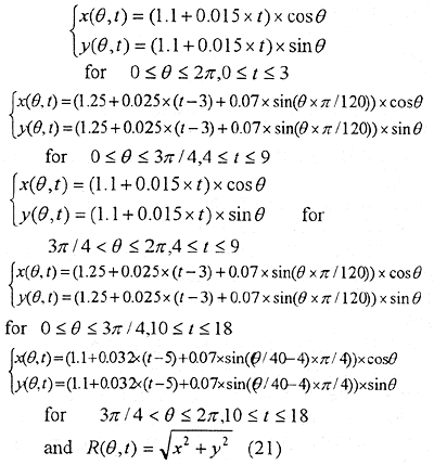
In order to plot the frost growth more explicitly as shown in the Figures in this section, the original frost shape 儭2(x,y,t) is transformed as 儭2(R, 兤, t). The unknown boundary configuration on 儭2(R, 兤, t) is assumed to vary with R, 兤 and t as:
the exact plot for the boundary configuration is shown in Figure 3. We should note that the frost thickness can be obtained by using R(兤,t) minus Ri, here Ri = 1.1 represents the tube radius.
The inverse analysis is first performed by using 9 thermocouple measurements (referring to Figure 1 where the dots "仠" denote the sensor's location with thermocouple spacing 儮兤 = 40o. When assuming exact measurements (冃 = 0.0), and using initial guess 儭20 = 儭2 (R,兤,0) and stopping criteria 兠 = 0.001, the estimated function of 儭2(R, 兤, t) by using the CGM is shown in Figure 4. It can be seen from Figures 3 and 4 that the CGM obtained good estimation of frost growth.
The average relative error between exact and estimated values after 34 iterations (兠 = 0.001) is 0.32 % for the present case and the average relative error is defined as error % =
The above numerical experiments were concerned with exact measurements, however measurement errors will always be introduced in any real measurement. It is important to detect the influence of the measurement errors to the inverse solutions under the present algorithm.
Two different noises are introduced here. For the frst one we assumed that the error in the order of about 1 % average measured temperature is introduced according to equation (17), i.e. the dimensionless measured temperatures with errors 冃 = 0.3 are considered (since the absolute average measured temperature is about 30). Next, measurement error with 冃 = 0.9 is used. The inverse solutions using these inexact measurements as the simulated temperature measurements are shown in Figures 5 and 6, respectively.
By using these 1 % (冃 = 0.3) and 3 % (冃 = 0.9) measurement errors, the resultant average error of the inverse solutions is about 1.83 % and 4.51 %, respectively. This implies that the CGM is not sensitive to the measurement errors since the measurement errors did not amplify the errors of estimated boundary shape (the errors are in same order of magnitude). Therefore the present technique provides a good estimation.
The above test cases seem unrealistic, since too many sensors were used in the numerical experiments. Now the question arises, can the number of sensors be reduced with the present approach? Let us first take a look at the role of measured temperature played in CGM. The measurement temperatures at sensor locations represent a boundary. point heat flux that appeared in the adjoint equation (13). Therefore it is possible to reduce the number of boundary point heat fluxes even though it will influence the value of J'. Now the question is that will this strategy influence the accuracy of the inverse solutions? To answer this, the numerical experiment is proceeded to the next case by utilizing 儭20 = 儭2 (R,兤,0), M = 5 (as was shown in Figure 1 with "儮" dots) and stopping criteria 兠 = 0.001, in estimating 儭2(R,兤,t) with measurement error 冃 = 0.0. The inverse solutions in predicting 儭2 under such an assumption using the CGM is shown in Figure 7. The average relative error between exact and estimated values after 35 iterations is 3.2 %.
From the comparison of numerical data in Figures 4 and 7, it is seen that the inverse solutions in predictuing 儭2 with 9 sensors are better than that with 5 sensors. However, the latter case is already good enough to be accepted as the inverse solution. Thus the number of sensors can be reduced when the CGM is applied.
In order to show the estimated inverse solutions more clearly. Figure 8 shows the estimated 儭2 obtained from Figures 4 and 5 at time t = 5 and 16, respectively. The computational results are listed in Table 1 for reference.
Numerical Test Case 2:
In the second test case, the unknown boundary configuration along 儭2(R,兤,t) is assumed to vary with R, 兤 and t as:

The exact plot for the boundary configuration is shown in Figure 9.
The inverse analysis is first performed by using 9 thermocouple measurements, 冃 = 0.0 and initial guess 儭20 = 儭2 (R,兤,0). The estimated function of 儭2(R,兤,t) is shown in Figure 10. The average relative error between exact and estimated values using 兠 = 0.001 for the present case is 0.4 %. It can be seen from Figures 9 and 10 that the CGM obtained good estimation of 儭2(R,兤,t).
Next we assumed that the error in the order of about 1 % average measured temperature is introduced according to equation (17), i,e. the dimensionless measured temperatures with errors 冃 = 0.3 are considered (since the absolute average measured temperature is about 30).