For the purpose of the failure analysis, it will be useful to interpret TTF as a random variable T.

Mathematically, the state of the component [1], or system in general, can be expressed in equation (1). Fig. 1 shows the relation between the state variable X(t) and the time of failure T.

　

　

Where,

X(t) = the state variable represents the condition of component at time t.

　

Fig. 1 The state variable and the time to failure of a component

　

Time to failure, T, of a component might follow one of several well-known distributions such as exponential, Weibull, normal or others distributions. The failure modeling can be derived by collecting a series of time to failure of the analyzed component. The illustration of a series of TTF of a component also can be seen in Fig. 1.

　

2.1. Cumulative Distribution Function And Probability Density Function

　

Assuming that TTF are continuously distributed with probability density function (pdf) f(t), then the probability that the component fails within the time interval (0,t) can be expressed into the following equation[1].

　

　

Where,

F(t) = the cumulative distribution function (CDF) of random variable T.

　

The pdf of random variable T can be derived from equation 2 simply by taking differential of F(t) with respect to t as shown in equation (3)[1].

　

　

2.2. Reliability Function

　

The reliability function R(t), which represents the probability that the component does not fail within the time interval (0,t] can be written into the following equation[1].

　

　

In term of reliability, equation (2) is also called as unreliability function and written as Q(t).

　

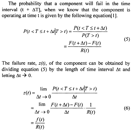
2.3. Failure Rate

　

　

2.4. Bathup Curve

　

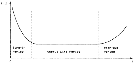
Fig. 2 shows a typical failure rate curve known as bathup curve. The curve consists of three different region of failure rate of a component. They are bum-in periods, useful life period, and wearout period respectively. As we can see in Fig. 2, the burn-in period is characterized by decreasing failure rate as a function of time or age. This can explained by the fact that there may be undiscovered defects in the components. The useful life period is characterized by constant hazard rate. In this region failures occur purely by chance and this is the only region in which the exponential distribution is valid. The wearout period is characterized by a rapidly increasing failure rate with time.

　

Fig. 2 Bathup curve [1]

　

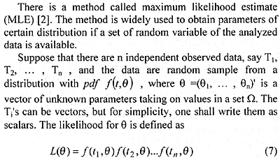
2.5. Maximum Likelihood Estimate (MLE)

BACK　　　CONTENTS　　　NEXT