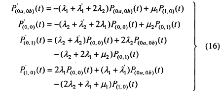
Now, if all failure states of the system are regarded as absorbing states, we have the following set of equations. Eq. (16), with initial condition [P(0a.0b) (0), P(0.0) (0), P(0.1) (0), P(1.0) (0)] = [0, 1, 0, 0] = [0, 1, 0, 0], by which the system reliability can be obtained.
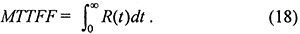
Laplace transform leads to the numerical solutions of P(0,0)(t) P(0a,0b) (t). P(0,1) (t) and P(1,0) (t). Then the system reliability and MTTFF are:
R(t) = P(0a,0b) (t) + P(0,0) (t) + P(0,1) (t) + P(1,0) (t),丂(17)
Similar to Section 3.1, Eq. (8) can be used to calculate system transient failure frequency. Under Mode II, Eq. (8) can be represented as the same with Eq. (9) where, both P(0,1) (t) and P(1.0) (t) are obtained from Eq. (12). The system mean failure times (MFN) in the interval (0, t) is then obtained by using Eq. (10). Furthermore, the MTBF of the system under steady state can be obtained by using Eq. (11).
丂
4. CASE STUDIES
丂
Numerical examples are given in order to solutions of system availability, reliability frequency under the two operation modes.
丂
4.1 Case of Mode I
Example: 兩1 = 0.005, 兩2 = 0.01, 兩'2 = O 006, 兪1 = 0.1, 兪2 = 0.06. There are two repair facilities.
R(t) = 1.04582exp(-0.004892t) - 0.02429exp(-0.09031t) - 0.02152exp(-0.1358t).
A(t) = 0.958845 + 0.054exp(-0.06548t) + 0.02752exp(-0.105t) - 0.02672 exp(-0.1268t) + 0.00424exp(-0.1569t) - 0.01553exp(-0.1954t) -0.005274exp(-0.21t) + 0.009515exp(-0.2203t) - 0.006603exp(-0.251t).
Mean failure times of the system up to time t, MFN is
MFN = 0.005504t+ 0.04229exp(-0.06548t) + 0.006263exp(-0.105t) + 0.01058exp(-0.1268t) + 3.843 亊 10-4exp(-0.1569t) + 0.00288exp(-0.1954t) + 7.681 亊 10-4exp(-0.21t) + 8.947 亊 10-4exp(-0.251t) -0.00 1241exp(-0.2203t) - 0.06282.
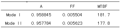
R(t) and A(t) are illustrated in Fig. 3 according to the above relations. Clearly in Fig. 3, R(t) and A(t) decrease with increasing of time t, and R(t) decreases fast. The system availability, failure frequency (FF) and MTBF under steady state are shown in Table 1.
丂
4.2 Case of Mode II
Example: 兩1 = 0.005, 兩1 = 0.003, 兩2 = 0.01, 兩'2 = 0, 006, 兪1 = 031, 兪2 = 0.06. Two repair facilities are used.
R(t) = 1.05377exp(-0.00502t) - 0.00943exp(-0.03033t) - 0.02118exp(-0.0889t) - 0.02316exp(-0.1347t).
A(t) = 0.957784 + 0.003441exp(-0.03088t) + 0.04756exp(-0.0646t) + 0.03196exp(-O.1033t) - 0.02696exp(-0.1268t) + 0.0041 24exp(-0. 1 567t) - 0.01556exp(-0.1954t) - 0.005182exp(-0.21t) + 0.00943 5exp(-0.2203t) - 0.006597exp(-0.251t).
Fig. 4 shows the results of R(t) and A(t) vs. time t through the above relations.
Mean failure times of the system up to time t, MFN, is given as follows
MFN = 0.005623t + 0.009215exp(-0.03088t) + 0.03832exp(-0.0646t) + 0.007428exp(-0.1033t) + 0.01068exp(-0.1268t) + 4.167 亊 10-4exp(-0.1567t) + 0.002887exp(-0.1954t) + 7.546 亊 10-4exp(-0.21t) + 8.944 亊 10-4exp(-0.251t) - 0.001231exp(-0.2203t) - 0.06937.
The system availability, failure frequency (FF) and MTBF under steady state are also shown in Table 1 in order to make a comparison with Mode I.
丂
丂
4.3 Discussion
Figs. 3 and 4, show clearly that a higher constant value of system availability holds under steady state even though the reliability is decreasing very fast in time. This is because repair rates are much greater than failure rates. Comparisons of the results obtained in Table 1 lead to the conclusion that Mode I is preferable to Mode II because it results in a higher value of system availability and lower failure frequency. From Figs. I and 2, and Eqs. (5) and (16), the system reliability is known to be identical under cases of that at most r (r = 1乣4) failed components can be under repair, that means, using two or more repair facilities does not make the system reliability increase for the 3-Out-of-4 system. However, the number of repair facilities does influence the system availability and failure frequency. Probably, the operating mode of a system or repair efficiency is a significant factor other than the number of repair facilities, which makes influence to system properties.
The results obtained above can be easily reduced to as for the hot or cold standby system, or the one with identical components.
Here, the system analysed consists of two kinds of units. If it is composed of three types of components and standby-priorities are assigned to them, we can infer that the system state transition diagram has three dimensions.