impaccts on dense water formation, essentially canceling their effect.
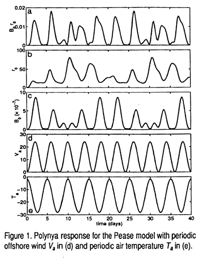
The effects of time-dependent wind and air temperature can be examined by solving (1) for specified Va and Ta. Figure 1 shows the response of a polynya over 40 days of forcing by a periodic offshore wind that varies between 0 and 24 m s-1 with a period of 4 days (Figure 1d), and a period air temperature that varies between -28.2 and -1.8亷 with a period of 5 days (Figure 1e). The resulting surface buoyancy flux (Figure 1c) varies over a wide range, from 0 to about 9亊10-7 m2s-3. It tends to be largest when the wind is strong and the air is cold. It vanishes when the air and water temperatures areidentical and is small when the wind vanishes. The polynya width (Figure 1b) is quite irregular, changing from a minimum of about 15 km to a maximum of about 80 km. As expected from the steady solutions, there is a tendency for B0 and r0 to vary inversely, al least on an event-by-event basis. That is, the width is small (large) when the buoyancy flux is large (small). The largest polynyas occur when B0 is small and Va. is nonzero (e.g. days 11 and 31). At these times the ice can be pushed far offshore before new ice production can close the polynya. Conversely, when the wind is weak and the buoyancy flux is strong, the polynya is quickly reduced to its minimum size (e.g, days 3 and 18).
Figure 1a shows the product B0r0. The large variability indicates that B0 and r0 are not as simply related as the steady part of (2) might have suggested. Total ice production obviously vanishes when B0 vanishes, but more interesting are the times when ice production is largest. These may occur when B0 is large and r0 is small (e.g. days 2 and 18) or when B0 and r0 are each in their mid-range of values (e.g. days 7 or 14). When the polynya is widest, ice production is small, although there is a sharp but short-lived increase in ice production as the buoyancy flux increases and rapidly reduces the polynya width (e.g. days 11-12).
丂
3. THE OCEAN RESPONSE
丂
To investigate the ocean response to a time-dependent polynya, the surface buoyancy flux and polynya width found from the Pease model (Figure 1) are used to force a pritmitive-equation numerical ocean model. The calculations follow closely the approach of Chapman and Gawarkiewicz (1997). The model is the semi-spectral primitive equation model described by Haidvogel el al. (1991). The model domain is a high-latitude, uniformly rotating, straight channel with periodic boundaries at the open ends. The domain is 100 km by 100 km with 1 km resolution in each direction. The ocean has uniform depth of 50 m, and nine Chebysev polynomials are used to resolve the vertical structure. Standard dynamical assumptions are made: rigid lid, no flow or density flux through solid boundaries, no stress at the solid boundaries or the surface, a Richardson-number based vertical mixing coefficient, convective adjustment to mix the density field whenever it is statically unstable, and small lateral Laplacian subgridscale mixing to ensure numerical stability. Further model details may be found in Chapman and Gawarkiewicz (1997). The calculation begins from rest with a homogeneous ocean. At time t=0, the surface buoyancy flux B0 (Figure 1c) is applied in a strip along the entire channel, adjacent to the coast and extending offshore a distance r0 (Figure 1b). The surface buoyancy flux is zero outside the polynya.
The ocean response is qualitatively identical to previous studies that used constant forcing: an unstable density front forms, eddies grow and separate from the polynya carrying dense water offshore, an equilibrium is reached in which the eddy flux balances the surface buoyancy flux. The primary difference is that the movement of t the edge of the polynya creates a region of gradually changing buoyancy flux exactly analogous to the forcing decay region used by Chapman and Gawarkiewicz (1997) to represent spatial variations in ice production. This is illustrated in Figure 2 which shows the surface buoyancy flux averaged over the entire 40 day period of forcing. A nearly constant buoyancy flux occurs within 12.5 km of the coast because the polynya is always open to that width (Figure 1c). The constant value is remarkably close to the average flux over Arctic polynyas estimated by Cavalieri and Martin (1994). 0ff shore of this region, the buoyancy flux decreases almost exponentially with an e-folding scale of about 7.5 km (dashed curve in Figure 2).