3.2 Identification using Optimization Algorithms

　

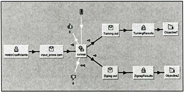
 The flow diagram reported in figure 3 represents, very simply, the scheme used to link the simulation program SIMSUP to the optimization tool FRONTIER.

　

　

 Reading the flow-diagram from left to right there are the following blocks:

- "Hydro Coefficients": hydrodynamic coefficients given in input and automatically modified by the optimization algorithm;

- "input_prova.cpm": file containing hydrodynamic coefficients in the format utilized by SIMSUP;

- "runner": this command starts the execution of SIMSUP in the version linked to FRONTIER;

- "Turning.out" and "ZigZag.out": output files of Turning Circle and ZigZag manoeuvres;

- "TurningResults" and "ZigZagResults": output macroscopic parameters typical of Turning Circle and ZigZag manoeuvres, obtained from the output files;

- "ObjectiveT" and "ObjectiveZ" : objective functions of Turning Circle and ZigZag manoeuvres.

　

 This scheme has been utilised already in order to perform automatically the sensitivity analysis. In order to identify the coefficients, the objective functions utilized are the same reported for the sensitivity analysis, modified in this case to measure the discrepancy between simulated manoeuvres and values obtained from experimental data.

 The identification procedure, schematized in figure 4, in general is structured as follows:

- Starting from an initial range of variation for the investigated coefficients a large number of combinations of hydrodynamic coefficients is generated randomly by the program and corresponding simulations are performed;

- The best 20 (about) solutions of this first calculation are assumed as input population for a second optimization made with a Multi Objective Genetic Algorithm (MOGA); the range of variation of the coefficients given in input is limited to the values corresponding to the best solutions identified by the previous step of calculation;

- The procedure is repeated iteratively with a sequence of MOGA reducing the range of investigation step by step until convergence is reached.

　

　

 As first step in order to validate the procedure it was applied to a 10°/10° ZigZag simulated manoeuvre and not to an experimental one, thus avoiding problems related to experimental data such as uncertainties, measurement errors and similar. The aim therefore was to obtain the coefficients used to generate the simulated manoeuvre starting from perturbed values for the full set of coefficients as established with the sensitivity analysis. In particular, since the optimization algorithm needs an initial estimate of the coefficients object of the identification, a perturbation of 10% from the value calculated by SIMSUP was assumed (representing the possible error which could be made by the use of regression formulae in a real case) and the range of variation for the first step of the calculations was set to ±35% from those initial perturbed values. In this case the coefficients were identified with an average error considered not satisfactory; this inaccuracy could be probably imputed to an ill-conditioning of the problem which could lead to cancellation effect between different coefficients, as was found in [9]; in order to lessen this problem, therefore, the calculations were repeated assuming the two manoeuvres simultaneously to constrain more the solution, and reducing the number of investigated coefficients to the five linear ones (Yv, Yr, Yd, Nv, Nr). The procedure was then applied assuming as objective function the sum of the two functions utilized for the sensitivity analysis (3) (4).

 With these second calculations the hydrodynamic coefficients were identified with a greater accuracy, and in particular there was a sensible improvement in the estimation of the most significant coefficients (Yd and Nr), estimated with an average error of 6% compared to the value of 12% previously obtained.

 Finally, if the simulations obtained with the initial values of coefficients are compared with those obtained with the optimized values estimated by the procedure previously described, they resulted nearly coincident and moreover, as further validation, similar results were obtained considering a 20°/20° ZigZag manoeuvre which was not directly involved in the identification procedure.

 The results of the comparison between the 20°/20°ZigZag initial manoeuvre and the corresponding simulated using the identified coefficient are reported in the next figure 5, where the curves are respectively pointed with "Simsup" and "Frontier".

　

　

 Once the procedure was validated it was applied to experimental data assuming in this case for the parameters indicated with "S" in the objective function no more the values estimated by SIMSUP, but the values obtained by experimental trials (in this study, in particular, data from full scale sea-trials were analyzed); the initial range for the values of the coefficients was now centered on the values estimated with SIMSUP regressions with a range of possible variation equal to ±35%.

 The values obtained for the coefficients investigated are reported in table 2 in the column named "Optim."; as it can be seen, they are in a good agreement with the PMM value, with an average error of 7%. In the next figures 6, 7 and 8 the time histories of manoeuvres, obtained by SIMSUP assuming the final coefficients identified by the optimization procedure (pointed in the diagrams with "Frontier") are compared to the experimental results (pointed with "Sperim.") and the simulations obtained assuming the values estimated by the regression formulae (pointed with "Simsup"). From the diagrams it can be observed that utilizing the values of coefficients obtained by the application of the identification procedure the estimation of the times histories of the manoeuvres resulted noticeably improved.

 In fact, for both the manoeuvres utilized in the identification procedure (35° Turning Circle and 10°/10° ZigZag) but also for a 20°/20° ZigZag manoeuvre the time histories simulated utilizing identified values result closer to experimental results than the ones obtained utilizing regression values.