|
4. ESTIMATION OF DIRECTIONAL WAVE SPECTRA
If ship motions are considered to be linear responses to incident waves, the cross spectrum of ship motions and the directional wave spectra are related by frequency transfer functions as follows:
where fe denotes encounter frequency, E(fe ,X) is the directional wave spectra based on encounter frequency, φij(fee,X) is the cross spectrum between the i-th and j-th components and Hi(fe,X) is the transfer function of the i-th component of the time series.
As the directional wave spectra should be expressed based on true wave frequencies for convenience, Εq. 7 must be transformed into true wave frequencies from encounter frequencies. Considering the triple valued function problem in the following seas, the discrete form of Εq. 7 can be expressed by the following matrix expression:
Φ(fe) = H(f01)E(f01)H(f01)*T+H(f02)E(f02)H(f02)*T+H(f03)E(f03)H(f03)*T (8)
where f01, f02and f03 are the true wave frequencies that correspond to the encounter frequency fe・Φ(fe) is the measured cross spectrum matrix, and H(f0i) and E(fOi) for (i=1,2,3) denote the matrices of transfer functions of the ship motions and directional wave spectrum at fO1, fO2 and f03respectively.
As Φ(fe) is a Hermitian matrix, Εq. 8 can be reduced to a multivariate regressive model expression using only the upper triangular matrix:
B = AF(x) + W (9)
where B denotes the cross spectrum vector, which is composed of real and imaginary parts of each element of Φ(fe),A denotes the coefficient matrix composed of products of the ship motion transfer functions, W is a Gaussian white noise sequence vector introduced for stochastic treatment and F(x) denotes the unknown coefficient vector that is composed of a discretized directional wave spectrum.
Based on the Bayesian modeling procedure, which was formulated by Akaike (1980), it is possible to evaluate unknown coefficients by minimizing the following cost function:
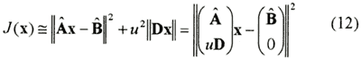
J(x) = ‖AF(x)- B‖2 + u2‖Dx‖ (10)
where D is the Gaussian smoothness prior distribution matrix, u2 is the hyperparameter and ‖a‖ denotes the norm of vector a.
In the actual calculations, the unknown vector should be expressed in the following form to avoid a negative wave spectrum:
F(x)T =(exp(xl)・・・exp(xJ)), exp(xj) = Ej(f0) (11)
As a consequence of the substitution of Εq. 11, the cost function becomes a non-linear equation that must be linearized for numerical calculation as follows;
where
and x0 is the initial value of unknown vector x.
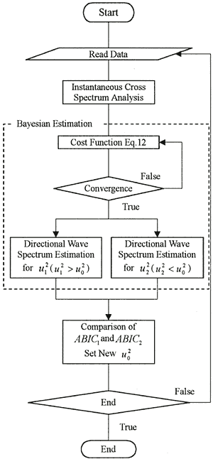
In the original Bayesian model algorithm, Εq. 12 is solved by the least squares method, with convergence achieved iteratively by substituting the newly calculated x into x0 and repeating. Furthermore, another iterative calculation is required to determine the optimum hyperparameter u2. The hyperparameter can be determined by minimizing Akaike's Bayesian information criterion (ABIC), which can be expressed as:
ABIC =-2log∫L(x|δ2)P(x)dx (13)
where L(x|δ2) and P(x) denote the likelihood function of the model and probability density function of the prior distribution.
To find the minimum value, ABIC is evaluated at various hyperparameter values, with each evaluation including an iterative calculation of Εq. 12. Therefore, most computational time is consumed by these iterative calculations.
In the proposed method, convergence of the iterative calculation for the hyperparameter is not achieved at every time step, but two different hyperparameters, one a little larger and the other a little smaller than the hyperparameter of the previous time step, are examined. The hyperparameter that is selected based on the ABIC is used as a starting point for the next time step. On the assumption that the seaway can be described by stationary stochastic processes, it is expected that convergence of the hyperparameter can be achieved gradually using the method proposed. A flow chart of this method is given in Fig.2.
5. SOME NUMERICAL TECHNIQUES FOR ON-BOARD TESTS
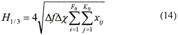
In application of the proposed method to actual merchant ships, of which only a minority is fitted with wave height sensors, analysis exclusive of wave height data can lead to over-estimates of wave power [1]. This kind of error occurs in the frequency range in which calculated response amplitude operators take small values but ship motions are measured. Although improving the accuracy of transfer functions is important, detailed data on the ship's hull form is unavailable in almost all cases. Therefore, the following new constraint condition is introduced into the Bayesian modeling procedure:
where H1/3 is the observed significant wave height, Δf and ΔX denote the resolutions of the discretization of wave frequency f and angle of encounter X.
FO and KO denote total numbers of discretizations.
This constraint is based on a relationship between the total volume of the directional wave spectrum and significant wave height. However, this constraint does not determine the total volume of the estimated spectrum directory, but is taken into account by the hyperparameter. Thus, the optimum directional wave spectrum can be estimated stably from the stochastic point of view.
Fig.2 |
Flow diagram of recursive Bayesian Estimation of directional wave spectra. |
|